Terravision / Services / 3D seismic interpretation / Demonstration
3D seismic interpretation: a demonstration on public data.
This is a demonstration of our 3D seismic interpretation service, run on a public dataset: the Parihaka 3D survey from the Taranaki Basin, offshore New Zealand. It is not client work, and we make no claim about the geology of any client's ground. We chose a public volume so that anyone can see what the deliverables look like and judge the quality for themselves.
Data: Parihaka 3D, Taranaki Basin, New Zealand. Courtesy of New Zealand Petroleum & Minerals (CC BY 4.0); SEG 2020 ML Interpretation Workshop subset, via Zenodo (doi 10.5281/zenodo.18988527). Public-dataset demonstration, not client work.
What we did
We worked through the volume in three stages.
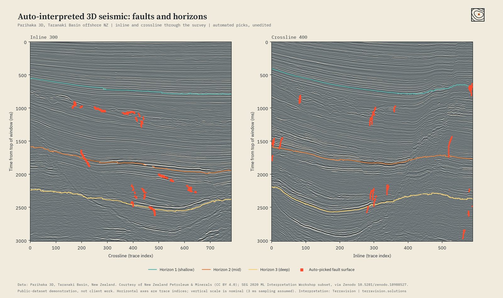
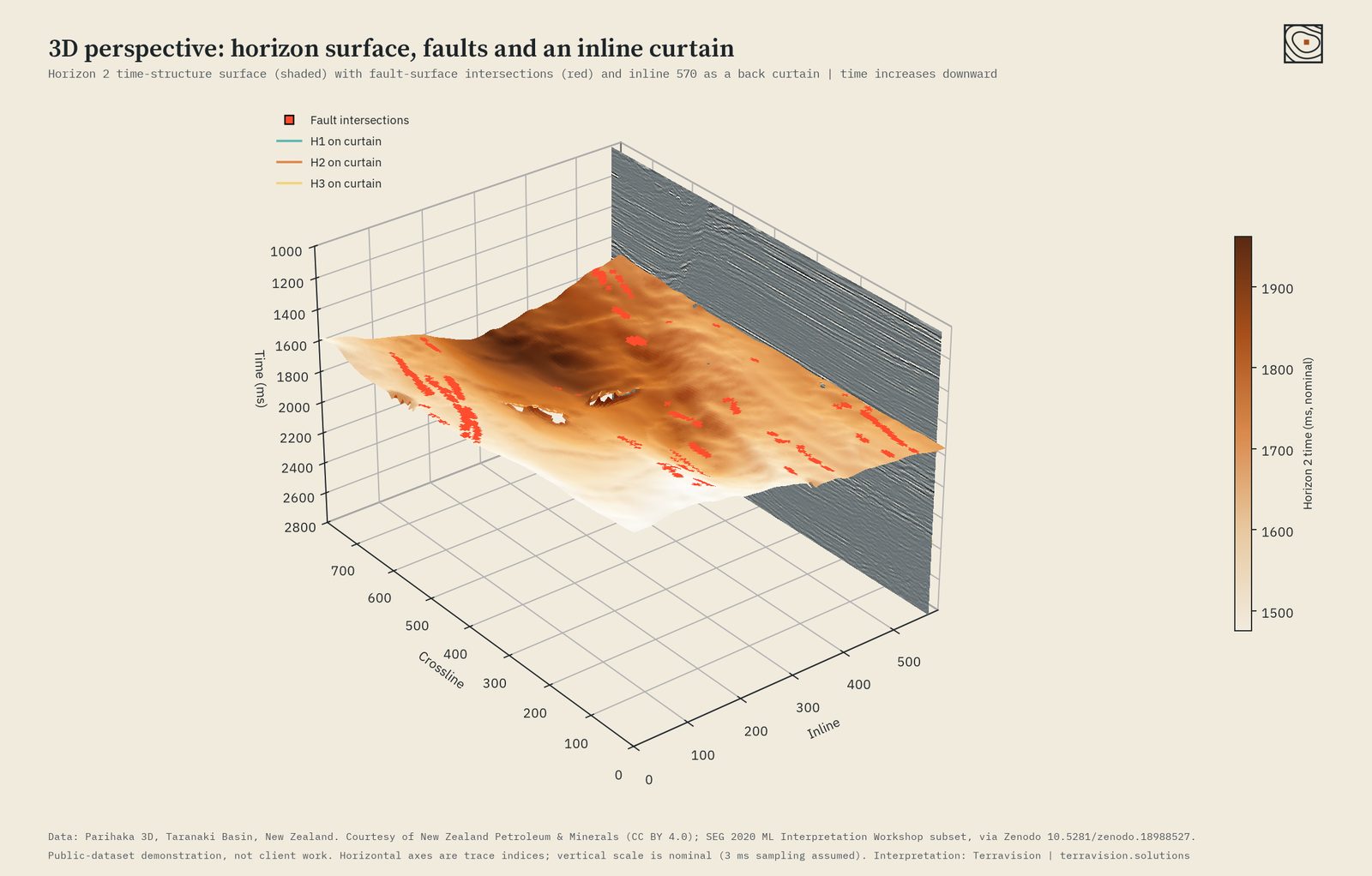
- Fault picking. We mapped fault surfaces through the whole 3D volume, not just on individual lines, and kept only the surfaces that are steep, continuous and plausibly planar. The result is a set of fault surfaces that can be read on any inline, crossline or time slice.
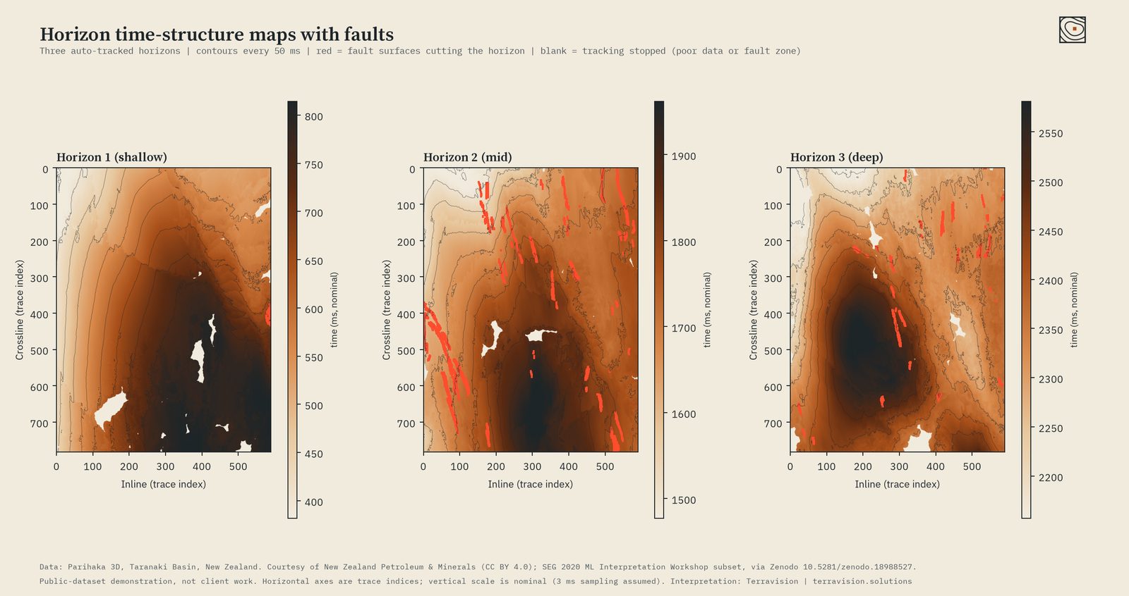
- Horizon tracking. We picked three reflectors (shallow, mid and deep) across the entire survey. Each horizon is tracked to about 97 to 99 per cent coverage. Gaps are left blank where the data is poor or a fault zone breaks the reflector, rather than filled with guesses.
- Time-structure maps. Each horizon is turned into a map of arrival time with contours every 50 ms and the fault intersections overlaid, so structural highs, lows and the fault pattern can be read at a glance. A 3D perspective view ties the surface, faults and a seismic section together.
The method in plain words
Seismic data is a stack of sound-echo images of the rock. Faults show up where those echoes are suddenly interrupted or offset.
- First, we measure which way the layers are dipping at every point in the volume. That tells us how the echoes ought to line up from one trace to the next.
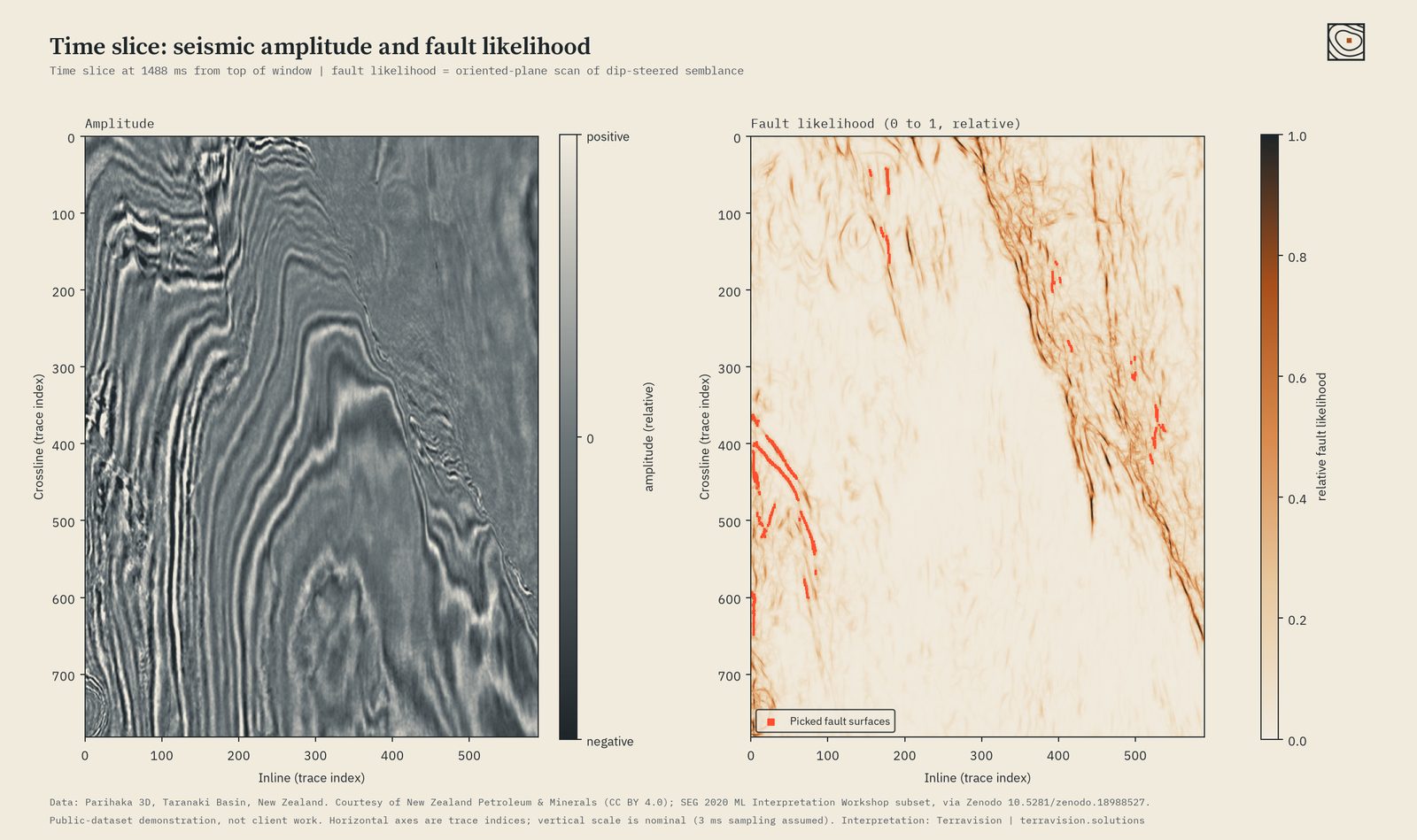
- We then check how well neighbouring traces agree with that expectation. Where they agree, the rock is continuous. Where they stop agreeing, something has broken the layers. This gives a “discontinuity” volume.
- To find faults, we scan that volume with tilted planes of many orientations and keep the strongest. The thin, planar, steep features that survive become the fault surfaces.
- For horizons, we pick a starting point on a clear reflector and grow outwards, following the layer's dip and matching the waveform from trace to trace. A final step checks that the whole surface is consistent, so small tracking errors do not build up across the map.
All of this uses conventional signal processing and geometry, and every pick is shown unedited, exactly as the workflow produced it.
What a client receives
- Fault surfaces and a fault-likelihood volume, supplied as standard files for import into your own interpretation software.
- Horizon grids for the agreed number of reflectors, with tracking-quality masks.
- Time-structure maps as PDF and image files, with contours and fault overlays.
- Annotated sections and time slices, like those shown here, for reports and presentations.
- A short methods and quality note saying what was picked, how well it tracked, and where we would not trust it.
Interpretation of this kind is a screening and planning aid. It does not replace the judgement of your own geoscientists, and we will say plainly where the data limits what can be picked. Horizontal axes in the figures are trace indices and the vertical scale is nominal.
Price
The final price depends on the size of the volume and the number of horizons. Send us a description of your survey and we will confirm the scope and price before any work starts. All prices in US dollars.
Have a volume and a question?
Describe your survey and what you need to know. We will say whether we are the right people for it, and confirm scope and price before any work starts.